Workdays in Excel

The WORKDAYS formula can be used in Excel to find what date is a given number of workdays from a set day, including that day. So in this example, the formula: =WORKDAY(A2,7)

. . . finds that seven days including from and after 12/24/2018 it will be January 2, 2019.

The WORKDAYS formula can also take account of holidays. In this example the holidays are listed in the range G2:G3. The formula: =WORKDAY(A3,7,G2:G3)

. . . finds that 7 workdays are in the period from 12/24/2018 through January 4, 2018, excluding the Christmas and New Year's Day holidays.

The holidays can be entered as serial numbers. 43459 is the serial number for 12/25/2018 and 43466 is the serial number for 1/1/2019.

The NETWORKDAYS formula will find the number of workdays in a given range. So in this example the formula:

=NETWORKDAYS(A2,B2)

. . .finds that there are 8 workdays in the range from 12/24/2018 to 1/2/2019.

With the NETWORKDAYS formula, don't enter the actual dates in the formula, but make reference to the cells which contain the dates, unless you use the serial number format.

=NETWORKDAYS(43458,43467)

It is also possible to insert dates into a formula under Formula . . . Date & Time . . . DATE

Enter the values and Excel will generate the correct serial number.

A new formula in this format:

=NETWORKDAYS(DATE(2018,12,24),DATE(2019,1,2))

. . . will be generated.

Half Deleted Characters

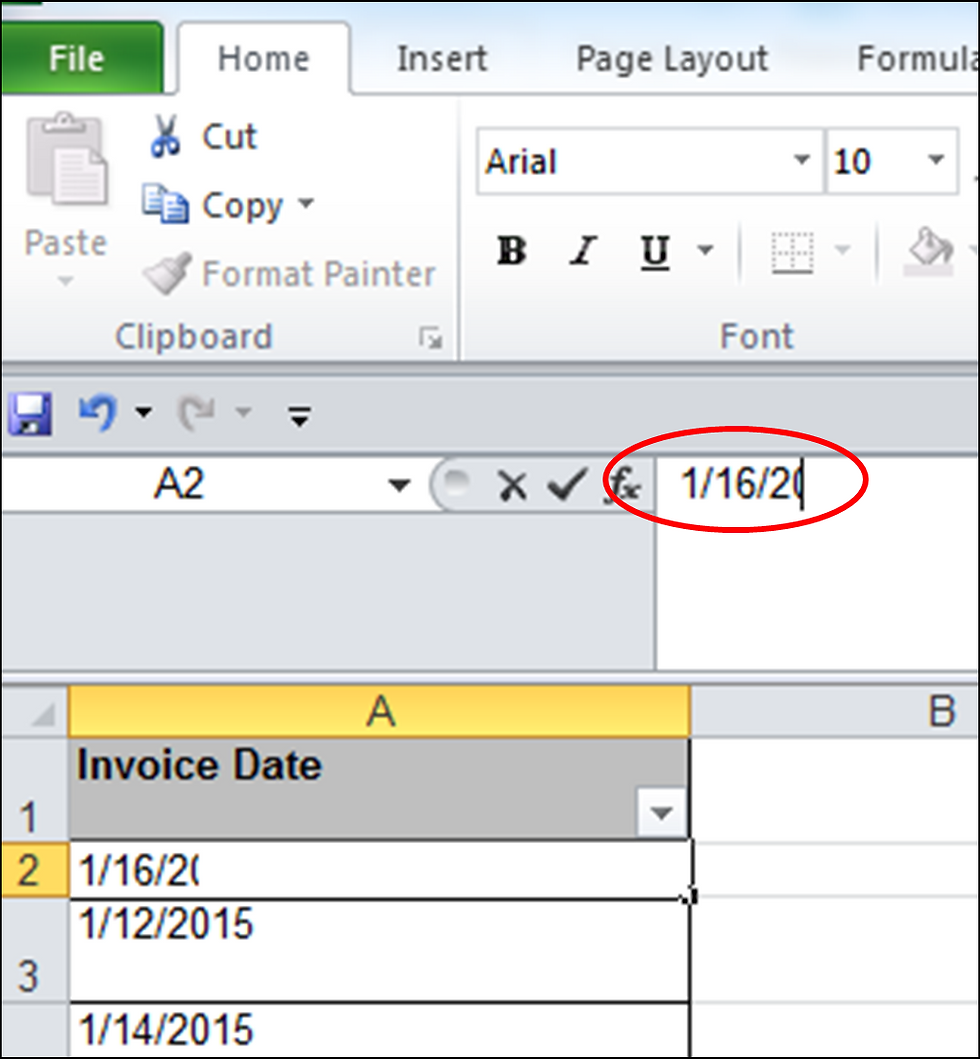
When editing data in a spreadsheet in Excel you may come across an odd problem in cells which have several blank cells at the end. If you remove those blank cells and begin to edit the rest of the characters, it will appear as though only half of a character gets deleted. After you are done editing, an extra character will be removed, and spaces will still exist at the end of the cell.

What's going on? Pasting the text into a text editor shows us what the problem is.

The text is enclosed in double quotes with spaces on either side which are not displayed in Excel. Remove the quotes and blank spaces and paste the data back into Excel and you will be able to format the data correctly.

Forecasting with Trendlines

Here's a follow-up to the Tip of the Night for January 20, 2019. Trendlines can be added to pivot charts to show the general trend between x and y values. Excel can forecast the trend for periods before or after those for which values are known.

To add a forecast, first select the data series on the chart (e.g., click the tops of the figures listed above bars in a bar chart). In the PivotChart Tools . . . Design submenu, select, 'Add Chart Element . . . Trendline . . . More Trendline Options . . . '. A 'Format Trendline' pane will open on the far right. As discussed in the Tip of the Night for January 20, 2019 select one of the six trendline options.

The section below will give you the option to set a forecast for the trendline X number of x axis units in the future or past.