Electronic Discovery Supply Chain Problems

The worldwide disruption in supply chains is impacting hardware used in electronic discovery. Solid state drives are in short supply for more than one reason. ABF (Ajinomoto Build-up Film) substrate is an insulation material used to protect chips. A Fortune Magazine article posted here, notes that Intel, Nvidia, AMD, and Broadcom all have had trouble getting a sufficient supply of the substrate.

Silicon wafers are needed for semiconductors. They form a base for integrated circuits. Semiconductor Engineering reported in September 2021 that, "Today, buyers of silicon wafers of many types face tight supply with rising average selling prices.".

Controllers for solid state drives are processors that run software. The power outages in Texas forced Samsung to shut down some of its SSD controller factories, according to Tom's Hardware.

There's a shortage of microchips across the board. Bloomberg has reported : "Lead times for Broadcom Inc.— a barometer for the industry because of its involvement across the supply chain—extended to 22.2 weeks, up from 12.2 weeks in February 2020."

Hot key for absolute reference

Just a very simple tip tonight, because Litigation Support Tip of the Night is exhausted and stressed out.

In Excel, if you want to automatically convert a cell reference to an absolute reference (a fixed reference that will remain the same when it's pulled down or across to other cells) press F4. Dollar signs will be added to the column letter and row number to make the reference absolute.

Creating a block chart in Excel

It's possible to set up a block chart in Excel in a few easy steps. This technique involves entering percentages in increments of one per cent in 100 cells on a worksheet.

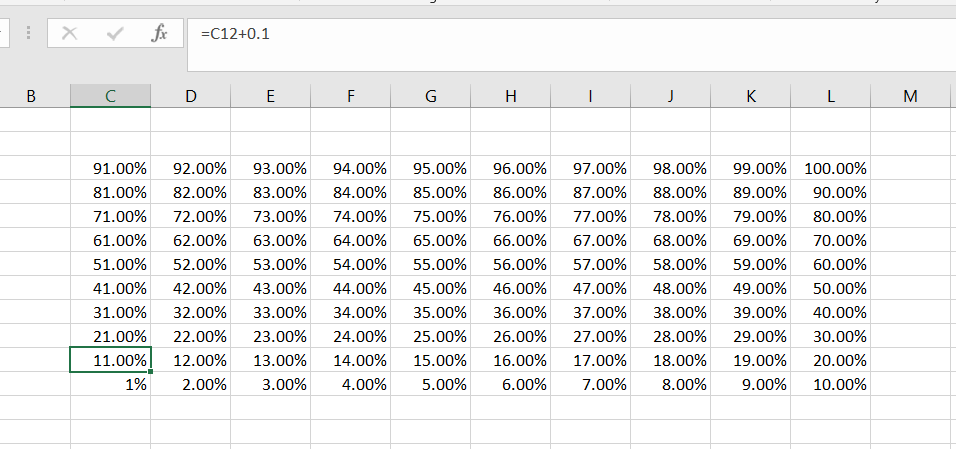
1. Begin by entering 1% in cell C12.

2. Enter C12 + 0.01 in cell D12 and pull it to the right so 1% to 10% is listed in columns C to L on row 12.

3. In cell C11 enter C12 +0.1, then pull the fill handle up so 11 % to 91 % is listed in in column C from row 11 to row 3.

4. Pull the formulas from column C over to column L so you have each percent point listed in a different cell:

5. You hide the results of these formulas by selecting the full range, and formatting the numbers to hide any positive, negative, or zero values by entering three semicolons in the custom field.

6. You can resize the cells into identical squares by carefully adjusting the row heights and columns widths to a set a number of pixels:

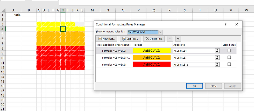
7. Select the lower half of the block staring from cell C8, and after selecting a new rule in Conditional Formatting using the type to 'Use a formula to determine which cells to format', enter the formula =C8<=$A$1

8. Now when percentages are entered in cell A1 which are less than 50%, a corresponding range of cells will be shaded in red.

9. Beginning at cell C5 select the range in the block for rows 5 to 7, and use the same type of conditional formatting rule with the formula: C5<=$A$1

10. Now when a percentage up to 80% is entered in cell A1, a range of cells from 51% to 80% will be shaded in orange.

11. Repeat this process for cells C3 through L4.

12. Now whenever a percentage is entered in cell A1, the block chart will fill up with red for the first 50%, orange for the next 30%, and yellow for the remaining 20%.

Thanks to Basement and Yard for posting this idea here.