Creating a block chart in Excel

It's possible to set up a block chart in Excel in a few easy steps. This technique involves entering percentages in increments of one per cent in 100 cells on a worksheet.

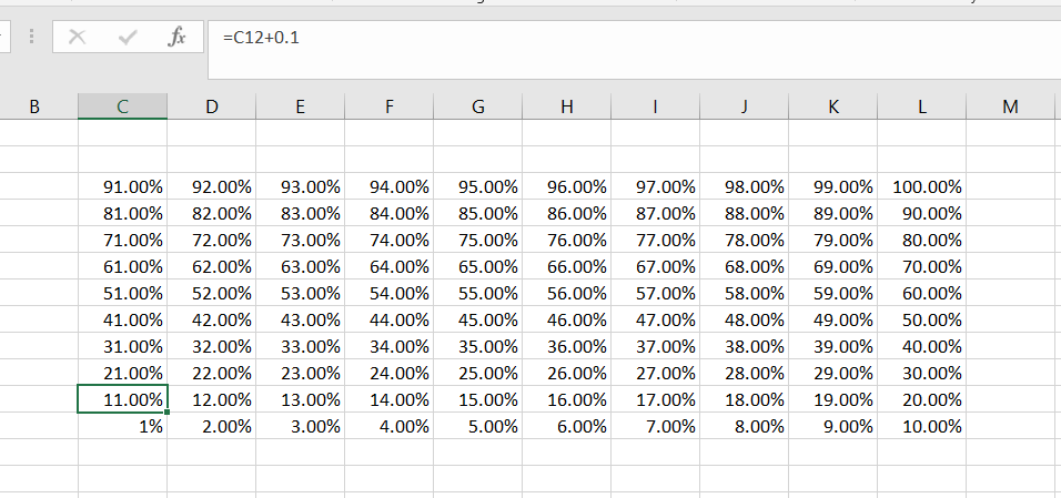
1. Begin by entering 1% in cell C12.

2. Enter C12 + 0.01 in cell D12 and pull it to the right so 1% to 10% is listed in columns C to L on row 12.

3. In cell C11 enter C12 +0.1, then pull the fill handle up so 11 % to 91 % is listed in in column C from row 11 to row 3.

4. Pull the formulas from column C over to column L so you have each percent point listed in a different cell:

5. You hide the results of these formulas by selecting the full range, and formatting the numbers to hide any positive, negative, or zero values by entering three semicolons in the custom field.

6. You can resize the cells into identical squares by carefully adjusting the row heights and columns widths to a set a number of pixels:

7. Select the lower half of the block staring from cell C8, and after selecting a new rule in Conditional Formatting using the type to 'Use a formula to determine which cells to format', enter the formula =C8<=$A$1

8. Now when percentages are entered in cell A1 which are less than 50%, a corresponding range of cells will be shaded in red.

9. Beginning at cell C5 select the range in the block for rows 5 to 7, and use the same type of conditional formatting rule with the formula: C5<=$A$1

10. Now when a percentage up to 80% is entered in cell A1, a range of cells from 51% to 80% will be shaded in orange.

11. Repeat this process for cells C3 through L4.

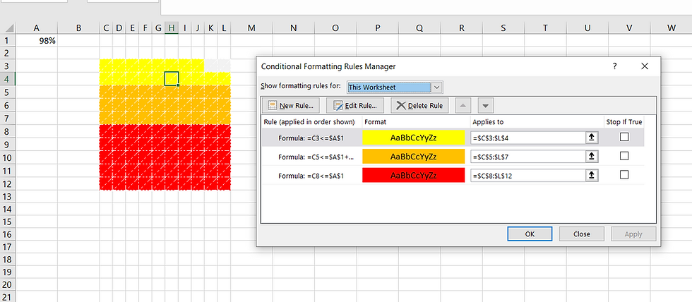
12. Now whenever a percentage is entered in cell A1, the block chart will fill up with red for the first 50%, orange for the next 30%, and yellow for the remaining 20%.

Thanks to Basement and Yard for posting this idea here.