Pivot Table Slicers

Slicers are an option for Excel pivot tables which allows you to use CTRL and SHIFT to select multiple options. If you have created multiple pivot tables on a worksheet you can use a slicer to apply filters to all of the tables at once.

To add a slicer, select any cell in the first pivot table. On the PivotTable Tools 'Analyze' tab select 'Insert Slicer' in the Filter group. Choose the field you want to filter by. A new box will appear that will allow you to select the entries you want to show in the pivot table.

To add the slicer to the second pivot table, select the Slicer itself. A new menu will open, 'Slicer Tools'. Under Options, click 'Report Connections' on the far left. You'll have the option to check off the second pivot table.

After you click OK the slicer setting will be applied to both pivot tables.

Controlling Iterative Calculations in Excel

Excel will usually give you an error message if you attempt to enter a circular reference. However formulas can refer to the cell in which they are entered if the option to perform iterative calculations is enabled.

Under File . . . Options . . . Formulas, check off 'Enable iterative calculation'. You have the option to set the maximum number of iterations, and the maximum change for each iteration. The maximum change sets how different the value of each iterative formula can be. The maximum number sets when Excel will stop performing calculations.

See this example:

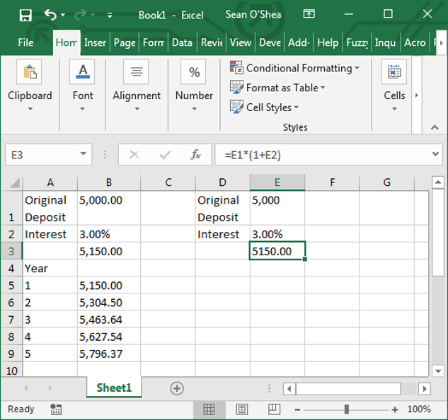
Here we see an Excel spreadsheet showing how an investment of $5,000, which accrues at a rate of 3% each year, grows. An absolute reference to the cell containing the interest rate is multiplied by the previous years total, and then added to the previous years total. Using this formula we can see that the original deposit grows to a total of $5,796.37 over five years.

With iterative calculations enabled, and set to a maximum of 4, we can get the same result in fewer cells.

Begin by entering the initial deposit in cell E1, the interest in cell E2, and then the formula, "=E1*(1+E2)" in cell E3.

Then in cell E1 enter a reference to the formula result.

As you can see you get the same result in cell E3 as in cell B9, showing the growth of the initial investment over five years.

Hiding Formulas

Tonight's tip is very simple. If you want to hide formulas in an Excel workbooks, take these steps:

1. In this example, we have a formula entered in column P.

2. Select column P, and then go to Home . . . Format . . . Format Cells

3. In the dialog box on the Protection tab, check off 'Hidden'.

4. As the note in the dialog box indicates in order for the change to take effect you then have to go to Review . . . Protect Worksheet and enter a password.

The formulas which are still present in column P will not be displayed in the formula bar.