INDEX MATCH divided is faster than Excel

The Tip of the Night for August 17, 2015, discussed using a nested INDEX formula as an alternative to VLOOKUP in Excel. Testing by Charley Kyd, discussed here, indicates using the INDEX and MATCH formulas in separate cells can get you much faster results. A nested INDEX MATCH formula only runs slightly faster than VLOOKUP, but when the INDEX and MATCH formulas are placed in separate cells, results can be obtained almost five times faster than with than with VLOOKUP.

So instead of entering the nested INDEX MATCH formula this way:

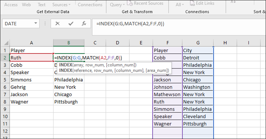
. . . enter the formulas in two columns searching for the row in the data range to be searched that the matches the unique value in the array you want a value from that range to be added to.

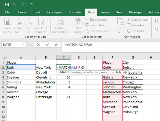
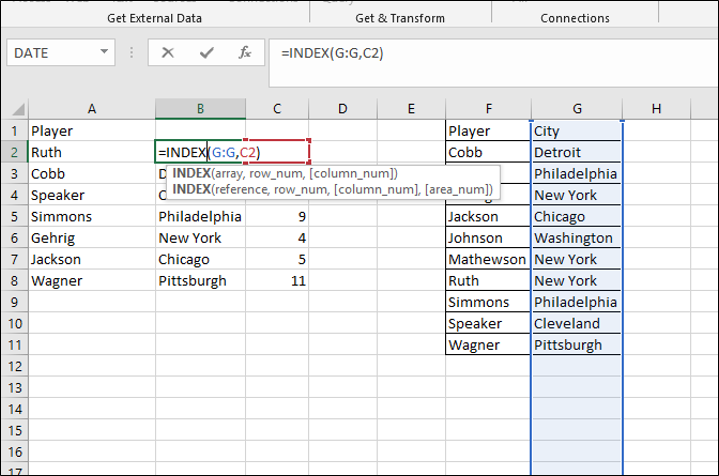
Then in a second column enter an INDEX formula that references the row number returned by the MATCH formula, but points to the column you want data pulled form.

Excel formula to pull column headings when given value is entered

Tonight's tip discusses how to use a formula in Excel to extract the column headings in a range of data for which a given value is entered. In this example we have a list of cities in column A, and columns B to E track which of these cities has a professional team for any one of the four major American sports.

This formula is entered in cell G2:

=IF(COUNTIF($F2:F2,INDEX(B$1:$E$1,MATCH("Yes",INDEX(B$2:$E$5,MATCH($A2,$A$2:$A$5,0),),0)))=0,INDEX(B$1:$E$1,MATCH("Yes",INDEX(B$2:$E$5,MATCH($A2,$A$2:$A$5,0),),0)),"")

The INDEX formula, with a nested MATCH formula, pulls an entry from the column headings in row 1, when the value 'Yes' is matched for the city in column A. The COUNTIF formula checks to see if the INDEX matches a value that the combined formula has found in the preceding cell. (The INDEX MATCH formula searches the full column range, not just one heading at a time, so there are no gaps in the list of heading hits.) The COUNTIF formula is written with the start of the range as an absolute cell reference, but the end of the range is not, so the range covered by the COUNTIF formula will expand as the formula is pulled to the right. The IF formula causes the result of the INDEX MATCH formula to be entered if the result is not already present.

Enter the formula two columns to the right of the data range to be reviewed. Pull it to the right using CTRL + R, for the same number of columns as exist in the data range, and then pull the formula down with CTRL + D. The values that get populated will only be those column headings that have "Yes" entered for a given city. You can then use the function discussed in the Tip of the Night for July 28, 2015, to combine the column headings and get a list of the sports in each city in a single cell like this:

Pivot Table Cache Limit

When the data used to generate a pivot table on your workbook is present inside the workbook, you can click any value in the pivot table to generate a complete list of the data used for this value on a new worksheet. However, if the data source for the pivot table was an outside file which is no longer linked to, when a value in the pivot table is clicked on you may receive this error message:

This "Not all source records have been copied" error will come up if the source data file had more than 65,536 rows. Excel creates a cache of the pivot table's outside data source (which shows the totals listed in the table itself based on the original complete data source) but only retains the first 65,536 rows of the data source.