Excel INDEX MATCH Formula to Pull Nth Value

You can use a modified INDEX MATCH formula to pull the second, third, fourth, the nth values from an array for the string you are searching for. So in this example:

=INDEX(B:B, SMALL(IF(A:A=D1,ROW(A:A)),3), 1)

. . . we search for the value entered in D1 in column A, and pull the value that appears in row B. So when we search for 'New York' like this:

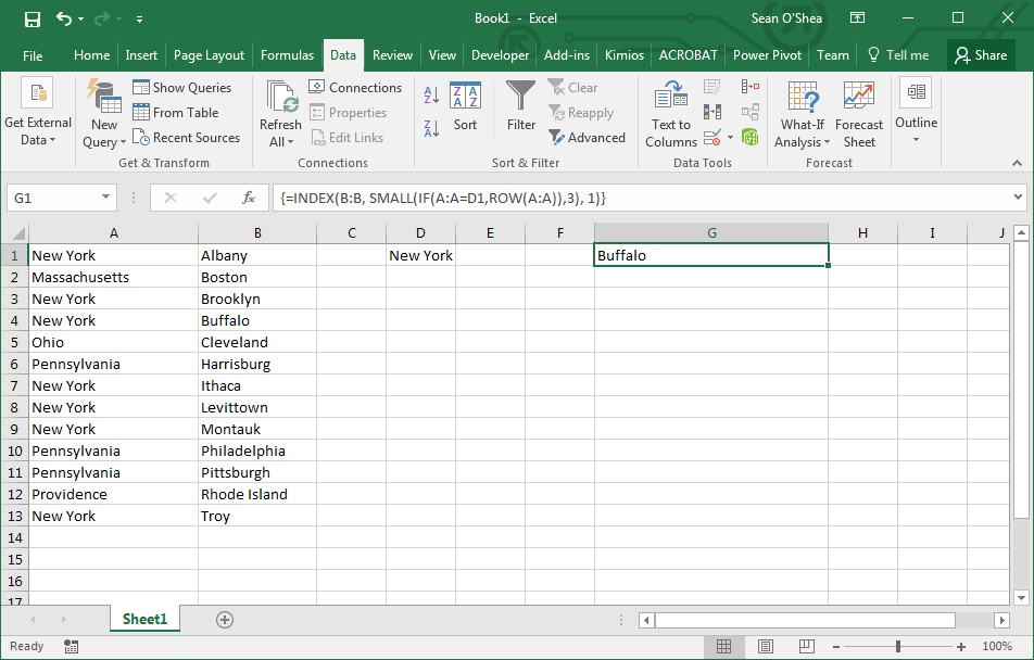
. . . we find the third New York city listed in column B. If we switch the '3' to a '4' at the end of the formula, we get the fourth city.

Note that this is an array formula so you have to press CTRL + SHIFT + ENTER when entering it and make sure that brackets appear around it.

Thanks to Mike Rickson for posting this formula here.