Use SUBTOTAL to Run Calculations on Filtered Data

A standard Excel formula like SUM will not be updated when a filter is applied to a worksheet.

If you want your calculations for a worksheet to change each time filters are set, use the SUBTOTAL function.

The SUBTOTAL function makes reference to multiple Excel formulas with numerical codes. Code 109 is for the SUM formula; 101 for AVERAGE;104 for MAX; 103 for COUNTA. Follow the code with the full range of data in a column. For example, =SUBTOTAL(109,L2:L22) or =SUBTOTAL(103,L2:L22)

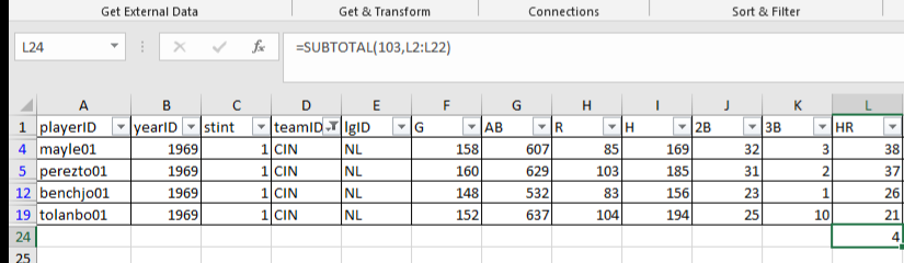
When the user filters the worksheet, only the calculation for the displayed rows will be returned.

Pull Data by Referencing Column Headings on Multiple Worksheets

This Tip of the Night shows how to search for column headings on multiple worksheets of an Excel spreadsheet, when the worksheets don't necessarily have columns with common headings in the same order. The worksheet to which the results of the formulas will be pulled, contains a reference number in one column, and a second column listing the name of the worksheet on which the reference number appears. A formula is used which will refer to those two columns and the column headings.

In this example, we want to add in the batting statistics for Rusty Staub on the first worksheet, when this data is listed on separate worksheets - each named with a different city he played in. The reference or control number is the year of a baseball season. Each worksheet with the data to be pulled has his stats in a different order:

Under the first column for which we want to pull data we enter this formula:

=HLOOKUP(D$1,INDIRECT("'"&$B2&"'!A:AZ"),MATCH($A2,INDIRECT("'"&$B2&"'!B:B"),0),FALSE)

This is a simple HLOOKUP formula which includes other formulas. Here's a breakdown

1. =HLOOKUP(D$1 - finds the value in the heading. An absolute reference is entered to the first row so when the formula is pulled down for subsequent years, it continues to enter the heading for each statistic.

2. INDIRECT("'"&$B2&"'!A:AZ") - this formula is used to enter worksheet reference in the HLOOKUP formula

3. MATCH($A2, - search for the control number - the season year in this example - so HLOOKUP knows which row to pull data from after it finds the heading.

4. INDIRECT("'"&$B2&"'!B:B"),0),FALSE) - the reference to the worksheet is entered again, to search on each worksheet for the control number. It is necessary for the reference number (the season year in this example) to appear in the same column on each worksheet.

Finding Numbers Stored as Text

A common problem in Excel is the need to convert numbers stored as text in a column to the number format. Numbers stored as text may not give correct results when they are referenced in formulas, and they will not necessarily sort in order with other numbers in the same column that are correctly formatted [although Excel should prompt you to sort them as numbers].

If you have a very long list of numbers, it may take a lot of scrolling back and forth to find where numbers stored as text begin in a column. If you find the first instance of numbers stored as text in a column, you can select from that cell to the end of the column, and click, 'Convert to Number'in the drop down menu on the right. All of the numbers in the column will be correctly formatted.

However in a column with thousands of numbers it may be hard to find the first instance of a cell with numbers stored as text. Use the ISTEXT formula in an adjacent column to identify which numbers are being read by Excel as text.

The formula will give the result "TRUE" for cells that are in the text format .